A word on financial returns
A brief introduction to financial returns
Posted by
Recent articles
Building a Hyperliquid Client in Python – Part III
Part III of the Hyperliquid client series covers private API endpoints, secure EIP-712 signing, and comprehensive order management. It offers practical guidance for account functions, error handling, and safe Testnet experimentation before transitioning to Mainnet.
Why TRX and JST Have Held Up Better Than Much of the Market
TRX and JST performance has been resilient in 2006 while most of the markets have faced challanges.
Building a Hyperliquid Client in Python – Part II
This hands-on continuation of the Hyperliquid client series focuses on implementing and using public /info endpoints. It details key data retrieval functions such as funding rates, candlesticks, and order books, and establishes a foundation for robust, production-ready API interactions.

Introduction
When analyzing financial assets, understanding how to measure returns is essential. There are three primary ways to calculate price changes, each with its own advantages and limitations.
As in all my blogs, I aim to make this blog both accessible to beginners and engaging for experienced investors.
Main types of returns
Arithmetic returns (straight price changes)
Arithmetic returns represent the simple difference in price between two time periods:, where is the return and the price both at time t.
If, for example, you buy a stock at $100 and sell it at $110, the arithmetic return is , so you gained $10 per share.
Arithmetic returns are symmetric, meaning that if the price goes one day from $100 to $110 and then the next day back to $100, you get a symmetric straight return.
Arithmetic returns are intuitive, as they reflect the actual dollar gain or loss from buying and selling an asset. However, they are affected by changes in scale, meaning that as prices increase, absolute returns tend to become larger.
Relative price changes/percent returns
Relative price changes, , express gains or losses as a proportion of the initial price, making them useful for comparing returns across different assets. Percent returns are just relative price changes multiplied by 100.
Relative price changes are not symmetric. Using my previous example, if the price goes to $110 from $100 is a 0.1 (10%) return, but if the price goes from $110 to $100 it is a 0.091 (9.1%) return. Therefore a 0.1 (10%) gain followed by a 0.1 (10%) loss does not bring the asset back to its original value.
This asymmetry poses a problem when calculating average returns. Using my previous example again, the average return is . If I just told the average return you would think that there is a small gain when in fact the gain is zero. This is one of the main reasons why logarithmic returns are often preferred in statistical finance: they preserve symmetry and better reflect long-term compounded growth.
Additionally, percentage returns are sensitive to scale changes over extended periods.
Logarithmic returns (log returns)
Log returns, , address some of the limitations of the previous methods. They are symmetric, making them more suitable for statistical modeling, and they are not affected by scale changes.
Following, once again, our previous example and .
However, logarithmic transformations alter the statistical properties of the returns process, which can impact the calculus of certain variables. A notable case is the calculation of correlation between variables. Correlation is affected, in general, by nonlinear transformations and so logarithms, which are a nonlinear transformation, can, and probably will, significantly affect correlation.
Summary
In summary, each method has its place depending on the context, whether it's trading, risk analysis, or financial modeling. Understanding their differences helps traders and investors choose the most appropriate measure for their strategies.
Statistical Measures of Returns
Beyond just measuring returns, understanding the distribution of returns is crucial for assessing risk and investment performance. Four important statistical measures are mean, standard deviation, skewness, and kurtosis.
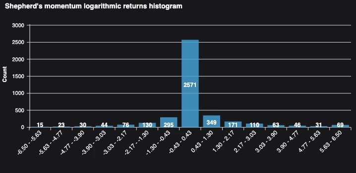
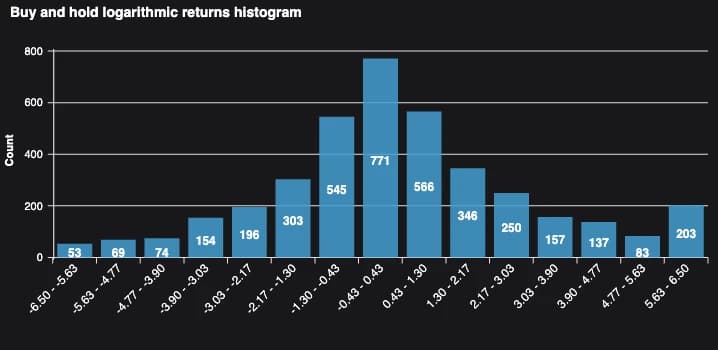
Let's consider, as an example, the two trading systems presented on my "Trading Bitcoin using a fast Shepherd's Momentum signal", blog: the Shepherd's momentum (SM) and buy and hold (B&H) trading strategies. The next table shows the mean, standard deviation, skewness and kurtosis calculated on logarithmic returns for both these strategies.
| Name | Shepherd's momentum | Buy and hold |
|---|---|---|
| Mean daily returns | 0.13 | 0.11 |
| Yearly standard deviation | 37.19 | 70.51 |
| Skewness | 0.84 | -0.89 |
| Kurtosis | 18.08 | 14.02 |
The logarithmic returns distribution for both strategies can be seen on the two following charts.
Mean
Mean or average is, as the name indicates, the average of a set of numbers. There are different types of means, for example:
- Arithmetic mean which is calculated by summing all values in a set and dividing by the total number of values in the set.
- Geometric mean which is calculated by multiplying all the values in a set and taking root of total number of values in the set.
- Harmonic mean which is calculated by dividing the total number of values in the set by the sum of the inverse of the set values.
Average returns may not mean a lot by itself as there is typically a proportional relation between return and risk. Higher risk leads to higher returns and lower risk leads to lower returns. Therefore is more usual for investor to prefer volatility adjusted indicators like the Sharpe Ratio or the Information Ratio
Standard deviation (volatility)
Standard deviation measures the dispersion of returns around their average. Higher standard deviation implies greater risk and uncertainty. As we can see in the table above the B&H as higher yearly standard deviation then SM. So B&H is riskier than SM because its returns fluctuate more. (check our Shepherd's volatility blog for more on volatility)
Skewness (asymmetry of returns)
Skewness measures whether the distribution of returns is biased toward gains or losses. A Positive skew means more frequent small losses, occasional large gains. A negative skew means more frequent small gains, occasional large losses (which is common in financial markets).
We can see that the B&H strategy has a negative skewness, which can indicate that the B&H strategy is prone to rare extreme losses (that can occur for instance during financial crises).
Kurtosis (distribution tails and extreme moves)
Putting it simply, Kurtosis measures how frequently extreme returns occur compared to a normal distribution. There two ways to present kurtosis: kurtosis and excess kurtosis. The kurtosis of a normal distribution is three. The excess kurtosis is zero. It is very usual to refer to excess kurtosis as just kurtosis and that is what I will do in this blog.
Distributions are said to be:
- platykurtic if kurtosis is less than zero,
- mesokurtic if kurtosis is equal to zero, the normal distribution is a mesokurtic distribution,
- leptokurtic if kurtosis is higher than zero.
Leptokurtic distributions, also known as fat-tailed distributions, exhibit more extreme returns, meaning that large gains and losses occur more frequently than in a normal distribution. Both SM and B&H returns are leptokurtic, but SM more so than the B&H, meaning occasional massive price spikes or crashes. In this particular case this is due to the fact that SM has many zero returns, consequence of being often out of the market. This makes the returns distribution very concentrated around the mean.
Want more insights on trading strategies and risk management? Subscribe to join the Trading Shepherd community today!