Forecasting Crypto Returns with a Simple MLP in PyTorch
A practical walkthrough of building a small multi-layer perceptron in PyTorch to forecast hourly crypto returns.
Posted by
 Joao Teixeira
Related reading
Trading Solana using a fast Shepherd's momentum binary signal
Explore Solana trading with Shepherd's Momentum. Compare binary signals to buy-and-hold using real market data.

Introduction
Neural networks are often presented as powerful forecasting tools, but in markets, the real question is not whether a model is sophisticated. The real question is whether it can extract a stable signal from noisy data that still behaves reasonably out of sample.
In this article, I take one of the simplest possible neural-network setups: a small Multi-Layer Perceptron (MLP) implemented in PyTorch, trained on hourly cryptocurrency data. The goal is not to build a production-ready trading system, but to show clearly how an MLP can be defined, trained, selected, and evaluated.
I use a very small architecture and a simple feature set: lagged volatility-adjusted returns. That makes it easier to understand what the network is actually doing, and whether the added nonlinearity is helping at all. Complexity is always easy to add; robust signal is not.
The results, as you will see, are mixed. I see it not as a failure but as part of the research process. A useful research process is not one that produces impressive backtests at any cost, but one that helps us separate promising ideas from noise. In that sense, even a modest experiment can be informative.
Note: I am a researcher, not a software engineer. The code provided is functional and tested, but it is intended as a research prototype rather than a production system.
This article is for educational purposes only. It is not investment advice, and nothing here should be interpreted as a recommendation to trade.
Trading futures is inherently a high-risk activity. You can lose more than your initial margin.
Introduction to Neural Networks and Multi-Layer Perceptrons
Neural networks were originally presented, at least in broad terms, as models inspired by the organization and functioning of the brain. The analogy should not be taken too literally, but it is still a useful starting point. Biological neurons receive signals through dendrites, process them in the cell body, and transmit signals through axons. The points of contact between neurons are called synapses. In an abstract way, artificial neural networks borrow this language and this general idea: inputs are received, combined, transformed, and then passed forward through the network.
Like the brain, however imperfect the analogy may be, a neural network must be trained before it can perform a useful task. In other words, it has to learn from data. Broadly speaking, there are two major learning paradigms: supervised learning and unsupervised learning. In supervised learning, the network is shown both the inputs and the correct answers, and learning takes place by comparing the network's output with the known target. In unsupervised learning, by contrast, the network is not given the correct answer in advance and must instead try to detect structure or patterns in the data on its own.
For readers interested in the intellectual roots of neural networks, a classic reference is Parallel Distributed Processing by Rumelhart, McClelland, and the PDP Research Group.
A Multi-Layer Perceptron, or MLP, shown in the following picture, is one of the simplest and most classical types of neural network.
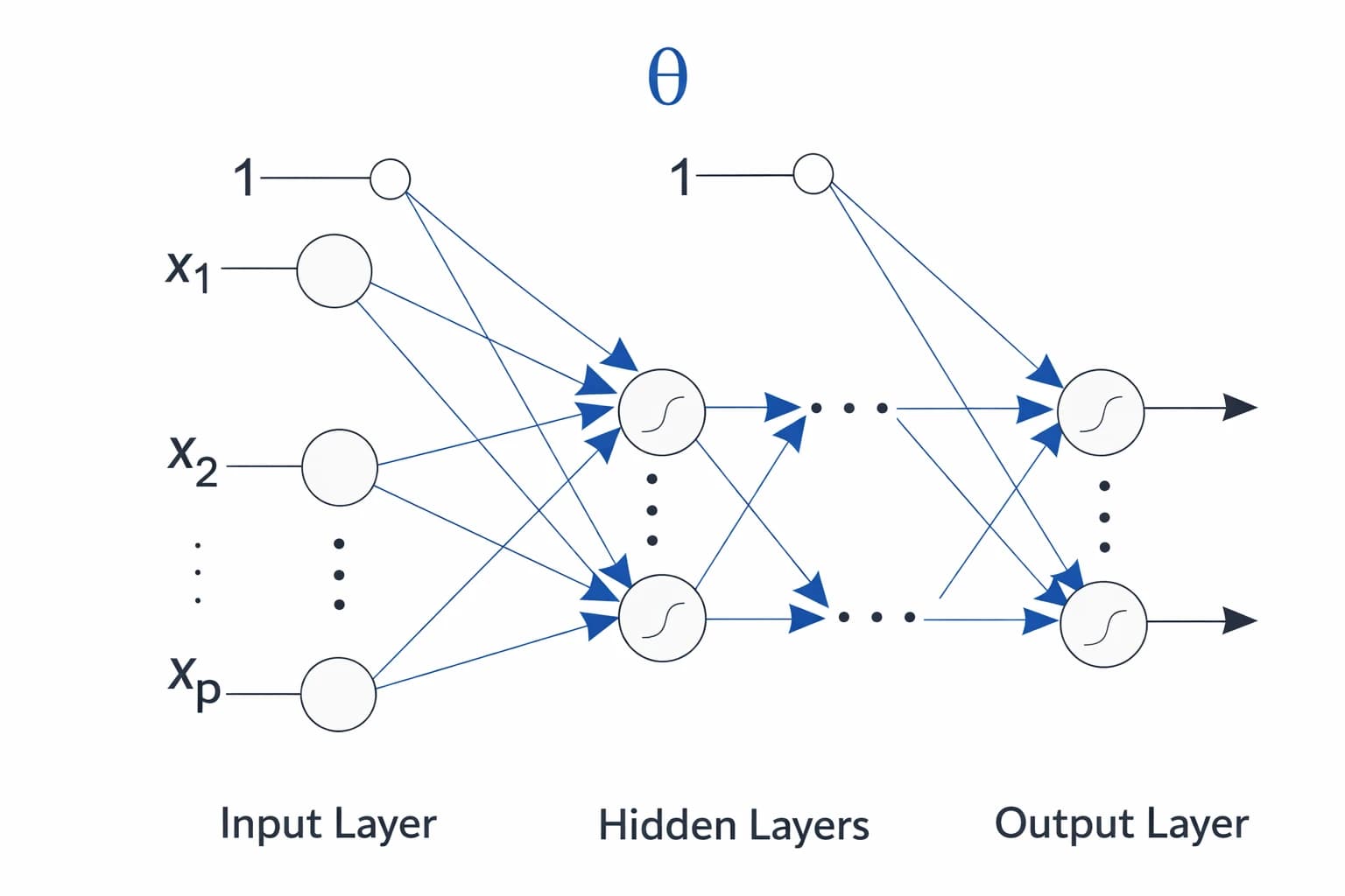
The MLP consists of an input layer, one or more hidden layers, and an output layer. Each neuron in one layer is typically connected to every neuron in the next layer, which is why an MLP is often described as a fully connected network.
Each hidden neuron computes a weighted combination of its inputs, adds a bias term, applies a nonlinear activation function such as tanh or ReLU (Rectified Linear Unit), and passes the result forward (see the next picture). By stacking these transformations, an MLP can represent nonlinear relationships between the inputs and the target.
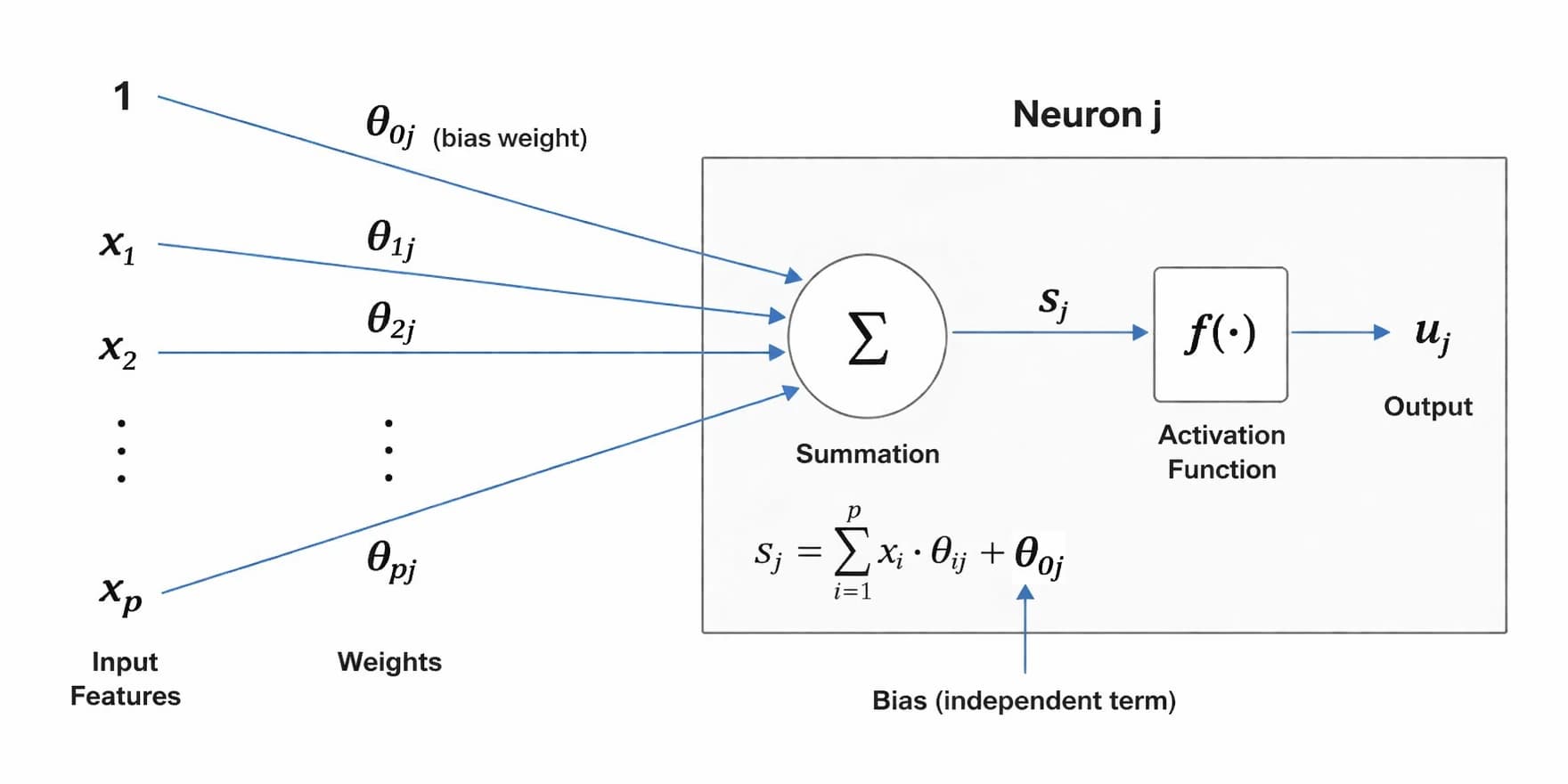
When studying neural networks, the MLP is a natural first step because the problem can be framed as a standard supervised-learning task: a vector of market features goes in, and a forecast for the next return comes out. Compared with more sophisticated architectures, an MLP is easy to understand, quick to implement, and a useful benchmark. If a small MLP cannot extract signal from the data, that is already informative. And if it does work, it provides a clean baseline against which more specialized architectures, such as 1D convolutional neural networks, can later be compared.
What is PyTorch?
PyTorch (https://pytorch.org) is an open-source machine learning and deep learning framework built around two core ideas: tensors and automatic differentiation. In practice, that means it gives you NumPy-like objects for numerical computation, plus the machinery to calculate gradients automatically, which is what makes neural-network training possible through backpropagation. The official documentation describes PyTorch as an optimized tensor library for deep learning on CPUs and GPUs, and its tutorials present it as both a NumPy replacement for accelerator-based computation and an automatic differentiation library for neural networks.
What makes PyTorch especially popular is that it feels very natural to Python users. You define models as nn.Module objects, express the forward pass in plain code, and rely on torch.autograd to compute gradients during training. Around that core, PyTorch provides practical building blocks such as torch.nn for layers and models, torch.optim for optimizers, and Dataset/DataLoader utilities for handling data pipelines, making it a flexible framework both for experimentation and for more structured production workflows.
PyTorch strikes a good balance between simplicity and power. You can start with a very small model written in just a few lines, but the same framework also supports more advanced workflows, from custom neural-network modules to GPU-based training. For someone learning neural networks, PyTorch is a natural choice: it is close enough to standard Python to be readable, but powerful enough to scale from a toy MLP to serious deep-learning models.
Model Identification
Model identification is about constructing models from experimental data. We need to define the network architecture: the feature set (the network inputs), intermediate layers (how many layers and how many neurons in each), and target definition (the network output).
Model identification then consists of comparing several versions of the same basic architecture. The main hyperparameter I varied was the number of neurons in the hidden layer.
Hyperparameters are configuration choices set before training begins. They determine the structure of the model or the way it is trained, but unlike the model's weights, they are not learned directly from the data. In my example, hyperparameters include:
- the number of hidden neurons (
hidden_dim), - the learning rate (
lr), - the batch size,
- the number of epochs (
n_epochs).
By contrast, the parameters of the model are the weights and biases that the neural network learns during training.
There are different, more or less complex methods, like for instance cross-validation, of model identification. I kept it simple: I divide my dataset into three subsets: training, validation, and test. Each candidate model was estimated on the training set and evaluated on the validation set, with validation performance determining the preferred specification.
After the best candidate had been identified, it was re-estimated on the training and validation data together, and its performance was examined on the test set. This procedure does not eliminate the danger of overfitting, but it imposes a useful structure on the research process and makes the results much easier to interpret.
This procedure is not just a technical detail, but a basic safeguard against fooling oneself. The training sample is the period on which the model's parameters are estimated. In other words, this is the data the neural network uses to learn the mapping from inputs to targets.
The validation sample serves a different purpose: it is used for model identification. Candidate specifications are trained on the training set and then compared on the validation set, with the validation results guiding choices such as the number of hidden neurons or the input configuration.
The test sample is reserved for the final out-of-sample assessment. It is the closest thing, within the research sample, to a simulation of how the model would have behaved on genuinely unseen data.
This distinction matters especially in finance, where the signal-to-noise ratio is low and the temptation to overfit is always present. A model can look impressive on the data used to estimate it and still fail once it is exposed to new market conditions. By separating the sample into training, validation, and test periods, the research process becomes more disciplined. The training set is used to fit the model, the validation set is used to select among competing specifications, and the test set is used only after those choices have been made. This does not eliminate overfitting, but it does make the results far easier to interpret and provides a much more realistic view of whether the model is capturing something persistent rather than merely adapting itself to noise.
Data Set
Working with cryptocurrency data is both easy and challenging. It is easy because the data is publicly available. It is challenging because, like most financial time series, the signal-to-noise ratio is very low.
For this article, I use Binance hourly data for five of the most liquid perpetual futures markets: BTCUSDT, DOGEUSDT, ETHUSDT, SOLUSDT, and XRPUSDT. One convenient way to download this data is from Binance Data.
The model uses 8 lagged volatility-adjusted returns as inputs to predict the next hour's volatility-adjusted return. The table below shows an example of the most recent data in the dataset.
| Market | Time | lag_7 | lag_6 | lag_5 | lag_4 | lag_3 | lag_2 | lag_1 | lag_0 | Target |
|---|---|---|---|---|---|---|---|---|---|---|
| ETHUSDT | 2026-03-22 18:00:00+00:00 | -0.2798 | -0.8507 | 0.9495 | -0.2982 | -0.0493 | 0.4134 | -0.0859 | -0.2185 | -0.6688 |
| SOLUSDT | 2026-03-22 18:00:00+00:00 | 0.0000 | -0.9169 | 0.8458 | 0.1012 | -0.2494 | 0.7982 | -0.2159 | -0.4855 | -0.5627 |
| ETHUSDT | 2026-03-22 19:00:00+00:00 | -0.8507 | 0.9495 | -0.2982 | -0.0493 | 0.4134 | -0.0859 | -0.2185 | -0.6688 | -0.8015 |
| SOLUSDT | 2026-03-22 19:00:00+00:00 | -0.9169 | 0.8458 | 0.1012 | -0.2494 | 0.7982 | -0.2159 | -0.4855 | -0.5627 | -0.3003 |
| ETHUSDT | 2026-03-22 20:00:00+00:00 | 0.9495 | -0.2982 | -0.0493 | 0.4134 | -0.0859 | -0.2185 | -0.6688 | -0.8015 | -0.4091 |
| SOLUSDT | 2026-03-22 20:00:00+00:00 | 0.8458 | 0.1012 | -0.2494 | 0.7982 | -0.2159 | -0.4855 | -0.5627 | -0.3003 | -0.6804 |
| ETHUSDT | 2026-03-22 21:00:00+00:00 | -0.2982 | -0.0493 | 0.4134 | -0.0859 | -0.2185 | -0.6688 | -0.8015 | -0.4091 | -1.1575 |
| SOLUSDT | 2026-03-22 21:00:00+00:00 | 0.1012 | -0.2494 | 0.7982 | -0.2159 | -0.4855 | -0.5627 | -0.3003 | -0.6804 | -1.3709 |
| ETHUSDT | 2026-03-22 22:00:00+00:00 | -0.0493 | 0.4134 | -0.0859 | -0.2185 | -0.6688 | -0.8015 | -0.4091 | -1.1575 | 1.4835 |
| SOLUSDT | 2026-03-22 22:00:00+00:00 | -0.2494 | 0.7982 | -0.2159 | -0.4855 | -0.5627 | -0.3003 | -0.6804 | -1.3709 | 1.6467 |
As you can see, each row corresponds to a given market at a specific hour. The input features are the lagged volatility-adjusted returns, and the target is the next volatility-adjusted return.
I divide the data into 3 sets: a training set containing 60% of the data, a validation set with 20%, and a test set with 20%. These sets are chronologically arranged: the training data occurs before the validation data, which in turn precedes the test set.
Imports
For this project, I will use the following imports:
import pandas as pd
import numpy as np
import matplotlib.pyplot as plt
import torch
import torch.nn as nn
from torch.utils.data import Dataset, DataLoader, TensorDataset
Defining and Running the Model
Model definition
I start by writing a class called SimpleMLP that defines a very simple feed-forward neural network in PyTorch. The model takes a vector of input_dim features as input, transforms them through a hidden layer with hidden_dim neurons, and returns a single output.
class SimpleMLP(nn.Module):
    def __init__(self, input_dim, hidden_dim):
        super().__init__()
        self.net = nn.Sequential(
            nn.Linear(input_dim, hidden_dim),
            nn.Tanh(),
            nn.Linear(hidden_dim, 1)
        )
    def forward(self, x):
        return self.net(x)
This class creates a new neural network by inheriting from nn.Module, which is the base class for all PyTorch models. nn.Sequential is a convenient way to stack layers one after another. Inside it we have:
nn.Linear(input_dim, hidden_dim): the first fully connected layer. It takes the input vector and maps it into a hidden representation of sizehidden_dim.nn.Tanh(): the activation function. It introduces nonlinearity, allowing the model to learn more complex relationships than a simple linear regression would. The tanh function squashes values into the range [-1, 1].nn.Linear(hidden_dim, 1)defines the output layer. It converts the hidden representation into a single number, which in our case is the model's prediction for the next volatility-adjusted return.def forward(self, x)defines how data flows through the model during prediction.- Finally,
return self.net(x)simply passes the input x through the sequence of layers defined above.
Loading the data into the model
The next helper function prepares the data so PyTorch can use it.
def create_dataloader(X_arr, y_arr, batch_size=256, shuffle=False):
    X_t = torch.tensor(X_arr, dtype=torch.float32)
    y_t = torch.tensor(y_arr, dtype=torch.float32)
    ds = TensorDataset(X_t, y_t)
    return DataLoader(ds, batch_size=batch_size, shuffle=shuffle)
Once the data enters the model, PyTorch needs to perform matrix multiplications, compute the loss, calculate gradients, update parameters, and run inference. This whole machinery works with tensors.
There are two common ways of setting up the tensors: torch.tensor(X_arr, dtype=torch.float32)and torch.from_numpy(X_arr).float().
TensorDataset(X_t, y_t) creates a dataset object that pairs each input row with its corresponding target row. Conceptually, if we have:
X_t[i] = features of sample[i]
and,
y_t[i] = target of sample[i]
then:
ds = TensorDataset(X_t, y_t)
creates something like a container where: ds[0] returns (X_t[0], y_t[0]), ds[1] returns (X_t[1], y_t[1]), etc. and len(ds) returns the number of samples. So it is basically telling PyTorch: these two tensors belong together row by row. This is useful because we don't want the training loop to be one giant loop. We want to iterate through the data in samples or mini-batches. TensorDataset is the object that organizes the data into that sample-wise form.
Finally, DataLoader(ds, batch_size=256, shuffle=True) takes this dataset and creates batches of samples, 256 at a time in this example. With shuffle=True, the samples are presented to the model in random order rather than chronological order. The data is now ready for the training loop, and the DataLoader will feed the dataset to the model one batch at a time.
Mini-batch training is computationally more efficient than using the entire dataset at once, and the randomness introduced by shuffling often helps the optimizer learn more robustly.
Note that shuffling is applied only within the training set. The train/test split itself should still respect time order, so that the model is always evaluated on genuinely future data.
Training the MLP
The model training is done by the train_model() function which trains the neural network for a fixed number of epochs and evaluates it on a validation set after each epoch.
def train_model(
                train_loader,
                val_loader,
                hidden_dim,
                n_epochs=25,
                lr=1e-3,
                device="cpu",
                verbose=False):

    input_dim = train_loader.dataset.tensors[0].shape[1]
    model = SimpleMLP(input_dim=input_dim, hidden_dim=hidden_dim).to(device)
    criterion = nn.MSELoss()
    optimizer = torch.optim.Adam(model.parameters(), lr=lr)
    history = []
    for epoch in range(1, n_epochs + 1):
        train_loss = run_epoch(model,
                              train_loader,
                              criterion,
                              optimizer=optimizer,
                              device=device)
        val_loss   = run_epoch(model,
                              val_loader,
                              criterion,
                              optimizer=None,
                              device=device)
        history.append({
            "epoch": epoch,
            "train_loss": train_loss,
            "val_loss": val_loss
        })
        if val_loss < best_val_loss:
            best_val_loss = val_loss
            best_epoch = epoch
            best_state_dict = copy.deepcopy(model.state_dict())

        if verbose:
            print(
                f"hidden={hidden_dim:2d} | epoch={epoch:2d} | "
                f"train={train_loss:.6f} | val={val_loss:.6f}"
            )

    final_val_loss = history[-1]["val_loss"]

    # restore best weights before returning
    model.load_state_dict(best_state_dict)

    return {
        "model": model,
        "history": history,
        "best_val_loss": best_val_loss,
        "final_val_loss": final_val_loss,
        "best_epoch": best_epoch,
        "best_state_dict": best_state_dict,
        "hidden_dim": hidden_dim
    }
This function takes:
train_loader: the training dataset, already split into batches.val_loader: the validation dataset, also in batches.hidden_dim: the number of neurons in the hidden layer.n_epochs=25: the number of times the model will go through the training set.lr=1e-3: the learning rate used by the optimizer.device="cpu": where the model runs, for example CPU or GPU.
This function is flexible: we can easily try different hidden-layer sizes, learning rates, or numbers of epochs.
After that I
- Instantiate the neural network and move it to the chosen device.
- Set the loss function to Mean Squared Error.
- Create the optimizer that will update the model parameters during training. Adam is one of the most commonly used optimizers in deep learning because it is usually stable and easy to work with.
- Loop the training process
n_epochstimes. Each epoch means one full pass through the training dataset. - Finally, run the same model on the validation data. But this time
optimizer=None, so the model is not updated. It is only being evaluated.
Essentially, the train_model() function is a wrapper around the full training process. It first infers the input dimension from the training data, builds a SimpleMLP with the chosen hidden-layer size, and defines both the loss function (MSELoss) and the optimizer (Adam). It then loops through the data for a fixed number of epochs, training on the training set and evaluating on the validation set after each epoch. The training and validation losses are stored in a history object so that we can later inspect the learning dynamics and compare alternative model configurations.
The function run_epoch() is the core engine of the training process: it runs the model over one full pass through a dataset and returns the average loss.
Depending on whether an optimizer is provided, it either trains the model on the batches in the loader, or evaluates the model on those batches without updating the weights. In both cases, it computes and returns the average loss over the full dataset.
def run_epoch(model, loader, criterion, optimizer=None, device="cpu"):
    if optimizer is None:
        model.eval()
    else:
        model.train()
    total_loss = 0.0
    total_n = 0
    for xb, yb in loader:
        xb = xb.to(device)
        yb = yb.to(device)
        preds = model(xb)
        loss = criterion(preds, yb)
        if optimizer is not None:
            optimizer.zero_grad()
            loss.backward()
            optimizer.step()
        batch_n = xb.size(0)
        total_loss += loss.item() * batch_n
        total_n += batch_n
    return total_loss / total_n
This function takes:
model: the neural network.loader: aDataLoaderthat yields batches of inputs and targets.criterion: the loss function, for example mean squared error.optimizer:Noneor the optimizer, if we want to train.device: where the model runs, for example CPU or GPU.
The key idea is that this same function can be used for both training and validation. Then the function:
- Instead of processing the entire dataset at once, the model works batch by batch
(xb, yb). - Moves data to the selected device (CPU or GPU).
- Takes the batch of inputs
xband produces a batch of predictionspreds. - If the optimizer is set, it performs the actual learning:
optimizer.zero_grad()clears old gradients,loss.backward()computes the new ones, andoptimizer.step()updates the weights.
The run_epoch() function performs one full pass through a dataset, one batch at a time. If an optimizer is provided, the model is put into training mode and its parameters are updated after each batch using backpropagation. If no optimizer is provided, the model is put into evaluation mode and only the loss is computed. The function keeps track of the loss across all samples and returns the average loss for the full epoch.
This function is the core engine of the training loop. It takes batches from the DataLoader, moves them to the chosen device, generates predictions, computes the loss, and, when training, updates the model weights. By using the presence or absence of an optimizer to switch between training and evaluation, the same function can be reused for both the training and validation phases.
Basic settings and running the model
The next code blocks bring everything together. They first set a few global parameters.
######################################
# BASIC SETTINGS
######################################
torch.manual_seed(123)

neurons_rng = range(1, 11)

device = torch.device("cuda" if torch.cuda.is_available() else "cpu")
The random seed improves reproducibility, meaning that if we rerun the script we should obtain the same or very similar results. neurons_rng = range(1, 11) defines the set of hidden-layer sizes I want to test. In this case, I arbitrarily chose models with between 1 and 10 neurons in the hidden layer. The device line chooses where the computations will run: GPU if available, otherwise CPU.
######################################
# PREPARE THE DATA
######################################

train_loader = create_dataloader(X_train, y_train, batch_size=256, shuffle=True)
val_loader   = create_dataloader(X_val, y_val, batch_size=256, shuffle=False)
test_loader  = create_dataloader(X_test, y_test, batch_size=256, shuffle=False)
Here we convert the train, validation, and test datasets into DataLoader objects. The training loader uses shuffle=True, so the training samples are presented in random order. This is standard in mini-batch training and often helps the optimizer converge more smoothly. The validation and test loaders use shuffle=False because at evaluation time we only want to measure performance.
######################################
# TRAIN MODELS
######################################

results = []
for hidden_dim in neurons_rng:
    result = train_model(
        train_loader,
        val_loader,
        hidden_dim=hidden_dim,
        n_epochs=25,
        lr=1e-3,
        device=device,
        verbose=False
    )
    results.append(result)
    print(f"hidden_dim={hidden_dim:2d} | validation MSE={result['best_val_loss']:.6f}")

# Pick model with smallest validation MSE
best_result = min(results, key=lambda d: d["best_val_loss"])
best_hidden_dim = best_result["hidden_dim"]
print("Best model according to validation set:")
print("hidden_dim =", best_hidden_dim)
print("validation MSE =", best_result["best_val_loss"])
This loop trains one model for each hidden-layer size in neurons_rng. For each value of hidden_dim, the code:
- Builds a new
SimpleMLP. - Trains it for 25 epochs.
- Evaluates it on the validation set.
- Stores the result in the results list.
- Prints the validation loss.
So this is a simple form of hyperparameter tuning. I am not changing the features or the optimizer, only the number of neurons in the hidden layer. The idea is straightforward: even with a very small network, the choice of hidden-layer size may affect performance, so we try several alternatives and keep the best one.
In summary, the final block of code performs a simple hyperparameter search over the size of the hidden layer. After fixing the random seeds for reproducibility and selecting the computation device (GPU if available, otherwise CPU), I create DataLoader objects for the training, validation, and test sets. I then train a separate SimpleMLP for each hidden-layer size from 1 to 10 neurons, always using the same number of epochs and learning rate. Each trained model is evaluated on the validation set, and the model with the lowest validation MSE is selected as the preferred specification.
Training results
The training results were:
hidden_dim= 1 | validation MSE=0.895753
hidden_dim= 2 | validation MSE=0.895775
hidden_dim= 3 | validation MSE=0.895784
hidden_dim= 4 | validation MSE=0.895640
hidden_dim= 5 | validation MSE=0.896111
hidden_dim= 6 | validation MSE=0.896151
hidden_dim= 7 | validation MSE=0.895692
hidden_dim= 8 | validation MSE=0.895589
hidden_dim= 9 | validation MSE=0.895456
hidden_dim=10 | validation MSE=0.895588

Best model according to validation set:
hidden_dim = 9
validation MSE = 0.895456100065112
The best model has 9 neurons in the hidden layer.
Model re-fitting
After selecting the preferred model specification using the validation set, the next step is to re-estimate its parameters on the combined training and validation data. The test set is then used only once, to assess how the final model performs out of sample.
In a live trading setting, the model would normally be re-estimated periodically as new data becomes available. A realistic out-of-sample evaluation should therefore mimic that process, for example through a walk-forward procedure in which the model is repeatedly re-fitted on past data and then tested on the subsequent unseen period.
Model Performance In- and Out-of-Sample
Next, I show the information ratio (IR) for the training plus validation set and also out of sample.
BTCUSDT: Training+validation IR=1.70, Out-of-sample IR=0.77
DOGEUSDT: Training+validation IR=2.84, Out-of-sample IR=0.14
ETHUSDT: Training+validation IR=1.65, Out-of-sample IR=-0.31
SOLUSDT: Training+validation IR=2.04, Out-of-sample IR=0.83
XRPUSDT: Training+validation IR=2.43, Out-of-sample IR=-0.10
Out-of-sample portfolio (equal weights) IR=0.30
The out-of-sample results are not great, and a few things must be noted. Firstly, this simulation is done cost-free. Second, I didn't perform any tests to establish the robustness of these results (by, for instance, changing the seed, slightly changing the out-of-sample set, or checking the out-of-sample performance using other numbers of neurons in the hidden layer).
Final remarks
We are used to the amazing job that Large Language Models (LLMs) do. These models have billions of parameters while my small model with just a few parameters did such a poor job.
The contrast with LLMs is not really a contradiction. The big difference is: in our case, we have limited data, low signal-to-noise, weak, unstable relationships, and not much redundancy.
LLMs are trained on an enormous amount of data, there is huge redundancy in language, the architecture is very well matched to the task, the pretraining objective gives a massive number of learning examples, and a lot of generalization is happening in a very dense representation space. So parameter count by itself is not the issue.
This article is not an invitation to trade. Also, it is not intended to provide trading advice. Trading involves risks, and readers are solely responsible for their trading decisions.
Trading futures is inherently a high-risk activity. You can lose more than your initial margin. This material is for educational purposes only.
Want deeper insights into risk and trading strategies? Subscribe to Trading Shepherd today and stay ahead of market volatility!"